Colorectal Cancer (CRC) Study
Soham Ghosh
2024-12-16
Last updated: 2024-12-17
Checks: 6 1
Knit directory: zinck-website/
This reproducible R Markdown analysis was created with workflowr (version 1.7.1). The Checks tab describes the reproducibility checks that were applied when the results were created. The Past versions tab lists the development history.
The R Markdown file has unstaged changes. To know which version of
the R Markdown file created these results, you’ll want to first commit
it to the Git repo. If you’re still working on the analysis, you can
ignore this warning. When you’re finished, you can run
wflow_publish to commit the R Markdown file and build the
HTML.
Great job! The global environment was empty. Objects defined in the global environment can affect the analysis in your R Markdown file in unknown ways. For reproduciblity it’s best to always run the code in an empty environment.
The command set.seed(20240617) was run prior to running
the code in the R Markdown file. Setting a seed ensures that any results
that rely on randomness, e.g. subsampling or permutations, are
reproducible.
Great job! Recording the operating system, R version, and package versions is critical for reproducibility.
Nice! There were no cached chunks for this analysis, so you can be confident that you successfully produced the results during this run.
Great job! Using relative paths to the files within your workflowr project makes it easier to run your code on other machines.
Great! You are using Git for version control. Tracking code development and connecting the code version to the results is critical for reproducibility.
The results in this page were generated with repository version d4297f5. See the Past versions tab to see a history of the changes made to the R Markdown and HTML files.
Note that you need to be careful to ensure that all relevant files for
the analysis have been committed to Git prior to generating the results
(you can use wflow_publish or
wflow_git_commit). workflowr only checks the R Markdown
file, but you know if there are other scripts or data files that it
depends on. Below is the status of the Git repository when the results
were generated:
Ignored files:
    Ignored:    .DS_Store
    Ignored:    analysis/.DS_Store

Unstaged changes:
    Modified:   .gitignore
    Modified:   analysis/CRC.Rmd
    Deleted:    analysis/CRC.html
    Modified:   analysis/Heatmaps.Rmd
    Modified:   analysis/IBD.Rmd
    Modified:   analysis/_site.yml
    Modified:   analysis/index.Rmd
    Modified:   analysis/simulation.Rmd
Note that any generated files, e.g. HTML, png, CSS, etc., are not included in this status report because it is ok for generated content to have uncommitted changes.
These are the previous versions of the repository in which changes were
made to the R Markdown (analysis/CRC.Rmd) and HTML
(docs/CRC.html) files. If you’ve configured a remote Git
repository (see ?wflow_git_remote), click on the hyperlinks
in the table below to view the files as they were in that past version.
| File | Version | Author | Date | Message |
|---|---|---|---|---|
| html | d4297f5 | ghoshstats | 2024-12-12 | Manually deploy website with existing HTML files |
| html | 3a96692 | Patron | 2024-06-18 | Updated CRC Study |
| Rmd | 116b71b | Patron | 2024-06-18 | Updated CRC study |
| html | ab6400d | Patron | 2024-06-18 | Build and publish the website |
| Rmd | a6c38f8 | Patron | 2024-06-18 | Add home, experiment, and simulation pages |
CRC Data Analysis
We applied zinck to meta-analyze five metagenomic
studies of CRC. The five studies correspond to five different countries
for the CRC data, which are named “AT” (Australia), “US” (USA), “CN”
(China), “DE” (Germany), and “FR” (France). The sample sizes are \(109\), \(127\), \(120\), \(114\), and \(104\), respectively, and the number of
cases and controls is roughly balanced in each study. We focus on all
the species whose relative abundances are more than \(0.2\).
##################### CRC data species level ##########################
#######################################################################
norm_count <- count/rowSums(count)
col_means <- colMeans(norm_count>0)
indices <- which(col_means > 0.2)
sorted_indices <- indices[order(col_means[indices],decreasing = TRUE)]
dcount <- count[,sorted_indices]

X <- dcount
Y <- ifelse(meta$Group=="CRC",1,0)
We train the zinck model on \(X\) using ADVI with an optimal number of
clusters (20). We generate the knockoff matrix \(\tilde{X}\) by plugging in the learnt
parameters \(\boldsymbol{\beta}\) and
\(\boldsymbol{\theta}\) into the
generative model.
fitCRC <- fit.zinck(X,num_clusters=20,method="ADVI",seed=1,boundary_correction = TRUE,
                    elbo_samples = 100,importance_resampling = FALSE,
                    prior_ZIGD = TRUE)
theta <- fitCRC$theta
beta <- fitCRC$beta
X_tilde <- zinck::generateKnockoff(X,theta,beta,seed=1) ## Generating the knockoff copy
We then move on to fit a tuned Random Forest model relating the augmented set of covariates with the outcome of interest \(Y\). The feature importance score used to construct the knockoff feature statistics \(W\) is the Mean Decrease in Gini Impurity.
filter_zinck <- zinck.filter(as.matrix(X),as.matrix(X_tilde),as.factor(Y),
                model="Random Forest",offset = 1,seed=1,mtry=28,
                rftuning=TRUE,metric = "Gini")

selected_species <- filter_zinck$selected


## Importance scores ##
W <- filter_zinck$W

## Threshold ##
T <- filter_zinck$T
Finally, we can visualize the importance of these selected species using the Feature Statistics obtained by contrasting the Random Forest importance scores of the original and the knockoff features.
### Creating the data frame with Feature Importance Statistics
data.species <- data.frame(
  impscores = sort(W[which(W>=T)], decreasing=FALSE) ,
  name = factor(names_zinck, levels = names_zinck),
  y = seq(length(names_zinck)) * 0.9
)

norm_count <- count/rowSums(count)
col_means <- colMeans(norm_count>0)
indices <- which(col_means > 0)
sorted_indices <- indices[order(col_means[indices],decreasing = TRUE)]
Xnorm <-norm_count[,sorted_indices]

# Calculate the column sums for cases and controls
case_sums <- colMeans(Xnorm[Y == 1, which(W>=T)])
control_sums <- colMeans(Xnorm[Y == 0, which(W>=T)])

# Determine colors based on the sum comparison
colors <- ifelse(case_sums > control_sums, "red", "blue")
The plot showing the identified species in order of decreasing importance is attached below.
# Create a data frame for plotting
data.species <- data.frame(
  impscores = sort(W[which(W >= T)], decreasing = FALSE),
  name = factor(names_zinck, levels = names_zinck),
  y = seq(length(names_zinck)) * 0.9,
  color = colors
)

plt.species <- ggplot(data.species) +
  geom_col(aes(impscores, name, fill = color), width = 0.6) +
  scale_fill_identity() +
  theme_bw() +
  ylab("Species") +
  xlab("Feature Statistic") +
  theme(
    axis.title.x = element_text(size = 22),
    axis.title.y = element_text(size = 22),
    axis.text.x = element_text(size = 18),
    axis.text.y = element_text(size = 18, face = data.species$fontface)
  )
print(plt.species)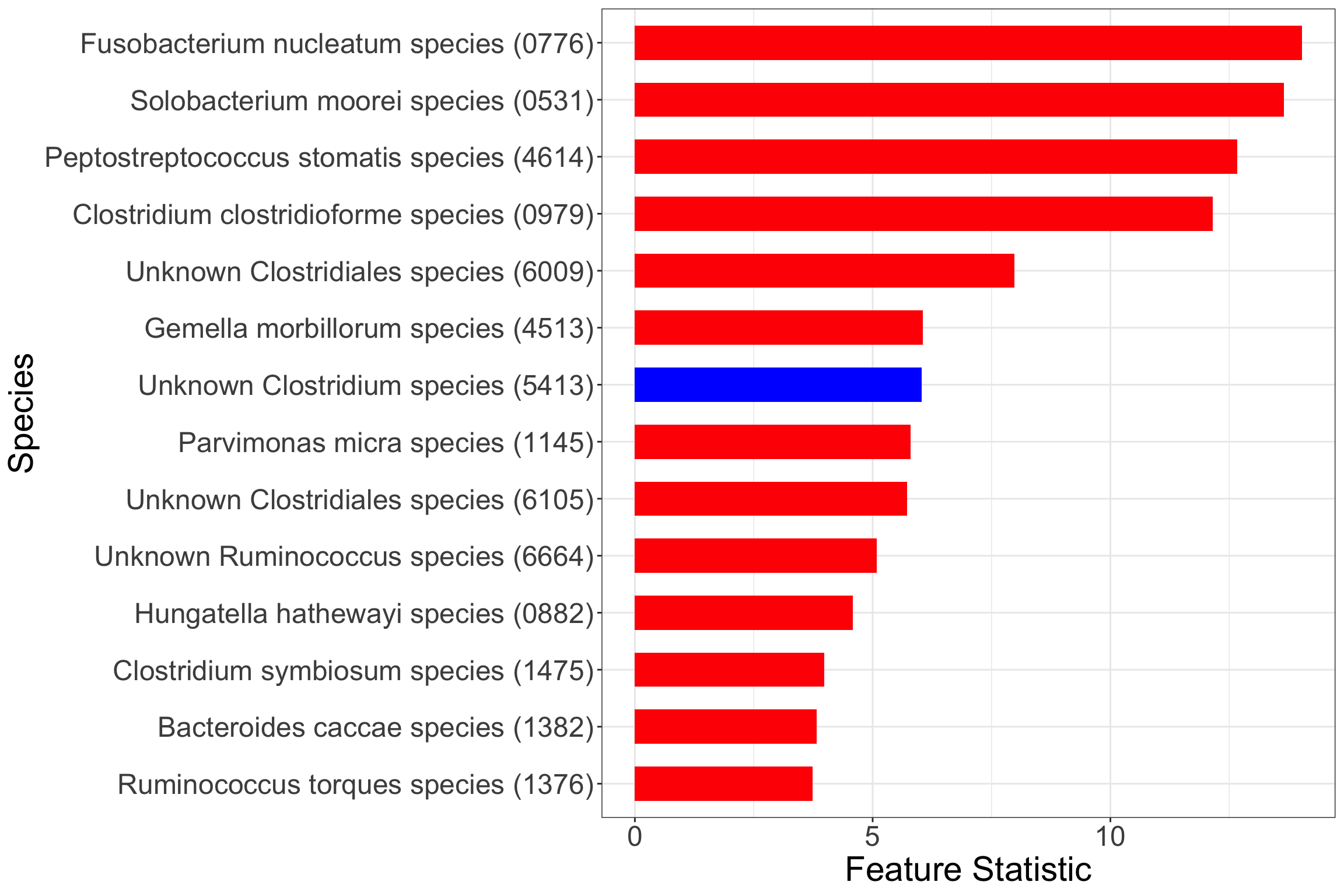
| Version | Author | Date |
|---|---|---|
| d4297f5 | ghoshstats | 2024-12-12 |
Note that the red colored bars indicate positive marginal association between microbial relative abundance and the odds of CRC, while blue indicate negative marginal association.
sessionInfo()R version 4.1.3 (2022-03-10)
Platform: x86_64-apple-darwin17.0 (64-bit)
Running under: macOS Big Sur/Monterey 10.16
Matrix products: default
BLAS: /Library/Frameworks/R.framework/Versions/4.1/Resources/lib/libRblas.0.dylib
LAPACK: /Library/Frameworks/R.framework/Versions/4.1/Resources/lib/libRlapack.dylib
locale:
[1] en_US.UTF-8/en_US.UTF-8/en_US.UTF-8/C/en_US.UTF-8/en_US.UTF-8
attached base packages:
[1] stats graphics grDevices utils datasets methods base
other attached packages:
[1] rstan_2.21.8 StanHeaders_2.21.0-7 ggplot2_3.4.2
[4] knockoff_0.3.6 reshape2_1.4.4 zinck_0.0.0.9000
[7] randomForest_4.7-1.1
loaded via a namespace (and not attached):
[1] sass_0.4.6 jsonlite_1.8.5 splines_4.1.3 foreach_1.5.2
[5] bslib_0.5.0 RcppParallel_5.1.7 highr_0.10 stats4_4.1.3
[9] yaml_2.3.7 pillar_1.9.0 lattice_0.21-8 glue_1.6.2
[13] digest_0.6.31 promises_1.2.0.1 colorspace_2.1-0 htmltools_0.5.5
[17] httpuv_1.6.11 Matrix_1.5-1 plyr_1.8.8 pkgconfig_2.0.3
[21] scales_1.2.1 processx_3.8.1 whisker_0.4.1 later_1.3.1
[25] git2r_0.32.0 tibble_3.2.1 generics_0.1.3 farver_2.1.1
[29] cachem_1.0.8 withr_2.5.0 cli_3.6.1 survival_3.5-5
[33] magrittr_2.0.3 crayon_1.5.2 evaluate_0.21 ps_1.7.5
[37] fs_1.6.2 fansi_1.0.4 pkgbuild_1.4.2 tools_4.1.3
[41] loo_2.6.0 prettyunits_1.1.1 lifecycle_1.0.3 matrixStats_0.63.0
[45] stringr_1.5.0 munsell_0.5.0 glmnet_4.1-7 callr_3.7.3
[49] compiler_4.1.3 jquerylib_0.1.4 rlang_1.1.1 grid_4.1.3
[53] iterators_1.0.14 rstudioapi_0.14 labeling_0.4.2 rmarkdown_2.22
[57] gtable_0.3.3 codetools_0.2-19 inline_0.3.19 DBI_1.1.3
[61] R6_2.5.1 gridExtra_2.3 knitr_1.43 dplyr_1.1.2
[65] fastmap_1.1.1 utf8_1.2.3 workflowr_1.7.1 rprojroot_2.0.3
[69] shape_1.4.6 stringi_1.7.12 parallel_4.1.3 Rcpp_1.0.10
[73] vctrs_0.6.5 tidyselect_1.2.0 xfun_0.39