Heatmaps
Soham Ghosh
2024-12-16
Last updated: 2024-12-18
Checks: 6 1
Knit directory: zinck-website/
This reproducible R Markdown analysis was created with workflowr (version 1.7.1). The Checks tab describes the reproducibility checks that were applied when the results were created. The Past versions tab lists the development history.
The R Markdown file has unstaged changes. To know which version of
the R Markdown file created these results, you’ll want to first commit
it to the Git repo. If you’re still working on the analysis, you can
ignore this warning. When you’re finished, you can run
wflow_publish to commit the R Markdown file and build the
HTML.
Great job! The global environment was empty. Objects defined in the global environment can affect the analysis in your R Markdown file in unknown ways. For reproduciblity it’s best to always run the code in an empty environment.
The command set.seed(20240617) was run prior to running
the code in the R Markdown file. Setting a seed ensures that any results
that rely on randomness, e.g. subsampling or permutations, are
reproducible.
Great job! Recording the operating system, R version, and package versions is critical for reproducibility.
Nice! There were no cached chunks for this analysis, so you can be confident that you successfully produced the results during this run.
Great job! Using relative paths to the files within your workflowr project makes it easier to run your code on other machines.
Great! You are using Git for version control. Tracking code development and connecting the code version to the results is critical for reproducibility.
The results in this page were generated with repository version d4297f5. See the Past versions tab to see a history of the changes made to the R Markdown and HTML files.
Note that you need to be careful to ensure that all relevant files for
the analysis have been committed to Git prior to generating the results
(you can use wflow_publish or
wflow_git_commit). workflowr only checks the R Markdown
file, but you know if there are other scripts or data files that it
depends on. Below is the status of the Git repository when the results
were generated:
Ignored files:
    Ignored:    .DS_Store
    Ignored:    analysis/.DS_Store

Unstaged changes:
    Modified:   .gitignore
    Modified:   analysis/CRC.Rmd
    Deleted:    analysis/CRC.html
    Modified:   analysis/Heatmaps.Rmd
    Modified:   analysis/IBD.Rmd
    Modified:   analysis/_site.yml
    Modified:   analysis/index.Rmd
    Modified:   analysis/simulation.Rmd
Note that any generated files, e.g. HTML, png, CSS, etc., are not included in this status report because it is ok for generated content to have uncommitted changes.
These are the previous versions of the repository in which changes were
made to the R Markdown (analysis/Heatmaps.Rmd) and HTML
(docs/Heatmaps.html) files. If you’ve configured a remote
Git repository (see ?wflow_git_remote), click on the
hyperlinks in the table below to view the files as they were in that
past version.
| File | Version | Author | Date | Message |
|---|---|---|---|---|
| html | d4297f5 | ghoshstats | 2024-12-12 | Manually deploy website with existing HTML files |
| html | 22a846b | Patron | 2024-06-19 | Updated Heatmaps |
| Rmd | 2ef880b | Patron | 2024-06-19 | Updated Heatmaps |
| html | 51a584c | Patron | 2024-06-18 | Changed Heatmaps |
| Rmd | 65fc471 | Patron | 2024-06-18 | Updated Heatmaps |
| html | ab6400d | Patron | 2024-06-18 | Build and publish the website |
| Rmd | a6c38f8 | Patron | 2024-06-18 | Add home, experiment, and simulation pages |
Comparing the Heatmaps for Original and Knockoff Sample Taxa Matrices
We demonstrate the ability of zinck to capture the
compositional and highly sparse nature of microbiome count data by
comparing the heatmaps of the original sample taxa matrix \(\mathbf{X}\) with its high quality knockoff
copy, \(\tilde{\mathbf{X}}\).
The CRC dataset contain \(574\) subjects (\(290\) CRC cases and \(284\) controls) and \(849\) gut bacterial species. Our analysis focuses on \(401\) species with an average relative abundance greater than \(0.2\) across all subjects. Then, we consider a toy setting with \(20\) randomly selected samples and \(30\) randomly selected CRC taxa at the species level. The sample library sizes vary between \(17\) and \(4588\), within an average library size of \(1329\). The zero-inflation level in the original sample taxa matrix is \(0.51\).
load("/Users/Patron/Documents/zinck research/count.RData")
norm_count <- count/rowSums(count)
col_means <- colMeans(norm_count > 0)
indices <- which(col_means > 0.2)
sorted_indices <- indices[order(col_means[indices], decreasing=TRUE)]
dcount <- count[,sorted_indices][,1:400]

set.seed(123)
selected_rows <- sample(1:nrow(dcount), 20)     ## Randomly select 20 subjects
selected_cols <- sample(1:ncol(dcount),30)      ## Randomly select 30 taxa
X <- dcount[selected_rows,selected_cols]      ## Resulting OTU matrix of dimensions 20*30
Next, we fit the ZIGD-augmented LDA model which is inbuilt within the
fit.zinck function of the zinck package, and
then use the posterior estimates of the latent parameters to generate
the knockoff copy.
model_zinck <- fit.zinck(X, num_clusters=13, method="ADVI", seed=2, boundary_correction = TRUE,prior_ZIGD = TRUE)
Theta <- model_zinck$theta
Beta <- model_zinck$beta
X_zinck <- generateKnockoff(X,Theta,Beta,seed=2)
We will now visualize the heatmaps of the original matrix and its
corresponding knockoff copy. The draw.heatmap function
applies an arcsinh transformation to the data for normalization and
better visualization of abundance patterns and zero inflation within the
sample taxa matrix. Note that, before displaying the heatmaps, we sort
the taxa in decreasing order of average sparsity among all the
subjects.
rownames(X_zinck) <- rownames(X)
draw.heatmap <- function(X, title = "") {
  reshape2::melt(asinh(X)) %>%
    dplyr::rename(sample = Var1, taxa = Var2, asinh.abun = value) %>%
    ggplot2::ggplot(., aes(x = taxa, y = sample, fill = asinh.abun)) +
    ggplot2::geom_tile() +
    ggplot2::theme_bw() +
    ggplot2::ggtitle(title) +
    ggplot2::labs(fill = "arcsinh\nabundance") +
    ggplot2::theme(
      plot.title = element_text(hjust = 0.5, size = 24),  # Increase font size here
      axis.title.x = element_blank(),
      axis.title.y = element_blank(),
      axis.text.x = element_text(size = 3, angle = 90),
      axis.text.y = element_text(size = 4)
    ) +
    viridis::scale_fill_viridis(discrete = FALSE, direction = -1, na.value = "grey") +
    theme(
      axis.title.x = element_blank(),
      axis.text.x = element_blank(),
      axis.ticks.x = element_blank(),
      axis.title.y = element_blank(),
      axis.text.y = element_blank(),
      axis.ticks.y = element_blank(),
      panel.grid.major = element_blank(),
      panel.grid.minor = element_blank(),
      panel.background = element_blank(),
      panel.border = element_blank(),
      legend.position = "none"
    ) +
    ggplot2::coord_fixed(ratio = 1)  # Fixing the aspect ratio
}

# Calculate the sparsity of each column for the Original OTU matrix
sparsity1 <- apply(X, 2, function(col) 1 - mean(col > 0))
sparsity2 <- apply(X_zinck, 2, function(col) 1 - mean(col > 0))

# Order the matrices by decreasing sparsity
X <- X[, order(sparsity1, decreasing = FALSE)]
X_zinck <- X_zinck[, order(sparsity2, decreasing = FALSE)]

heat1 <- draw.heatmap(X, "Original taxon count matrix")
heat2 <- draw.heatmap(X_zinck, "Zinck knockoff copy")
plot_grid(heat1, heat2, ncol = 2, align="v")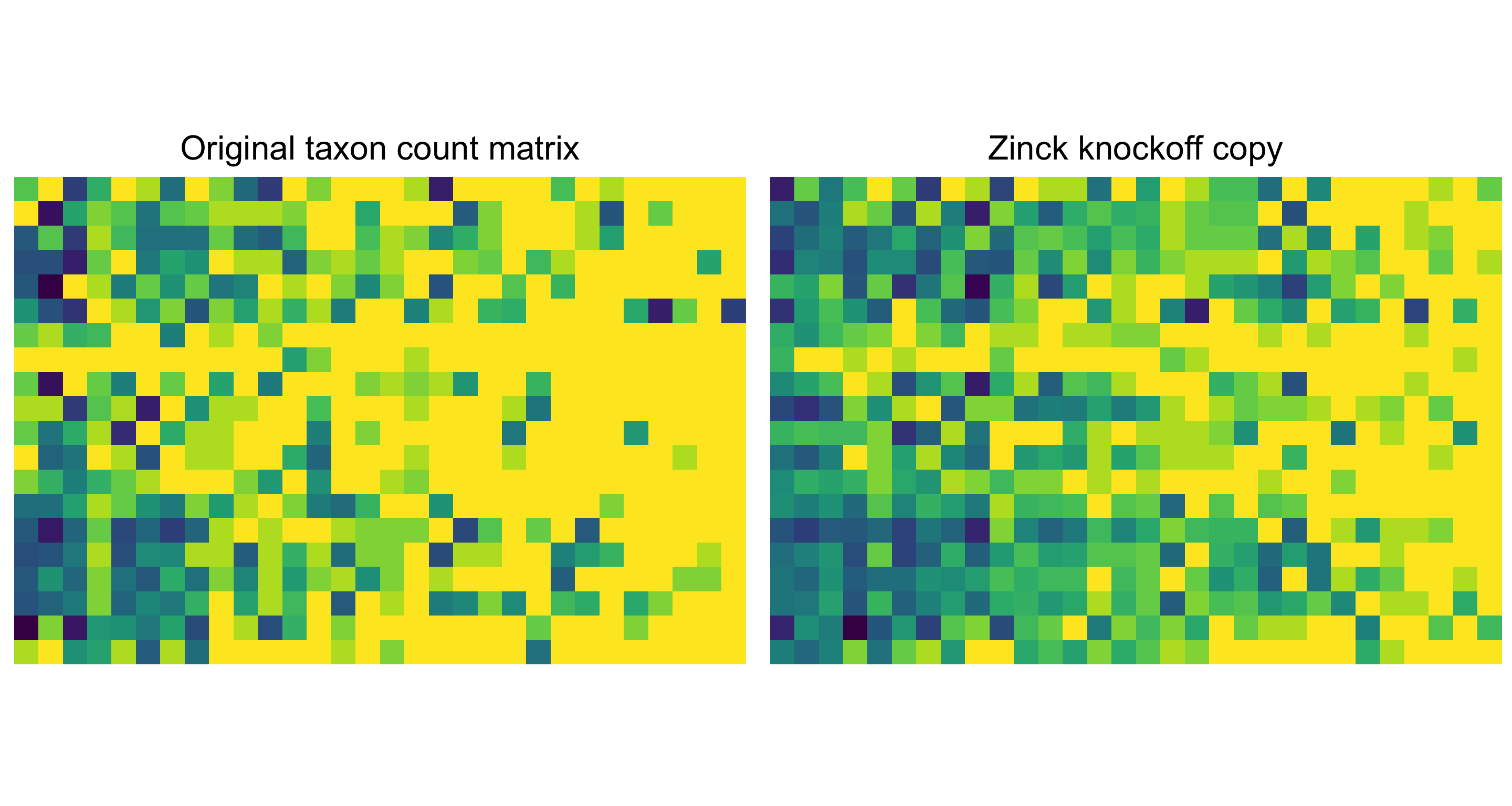
It is evident from the above heatmaps that the knockoff copy depicts most of the features corresponding to the original matrix, in terms of zero-inflation and compositionality. This underscores the fact that the knockoff copy preserves the underlying structure of the observed sample taxa count matrix.
sessionInfo()
R version 4.1.3 (2022-03-10)
Platform: x86_64-apple-darwin17.0 (64-bit)
Running under: macOS Big Sur/Monterey 10.16

Matrix products: default
BLAS:   /Library/Frameworks/R.framework/Versions/4.1/Resources/lib/libRblas.0.dylib
LAPACK: /Library/Frameworks/R.framework/Versions/4.1/Resources/lib/libRlapack.dylib

locale:
[1] en_US.UTF-8/en_US.UTF-8/en_US.UTF-8/C/en_US.UTF-8/en_US.UTF-8

attached base packages:
[1] stats     graphics  grDevices utils     datasets  methods   base

other attached packages:
 [1] cowplot_1.1.1        randomForest_4.7-1.1 gridExtra_2.3
 [4] glmnet_4.1-7         Matrix_1.5-1         reshape2_1.4.4
 [7] ggplot2_3.4.2        zinLDA_0.0.0.9000    dplyr_1.1.2
[10] knockoff_0.3.6       zinck_0.0.0.9000

loaded via a namespace (and not attached):
 [1] viridis_0.6.5        sass_0.4.6           jsonlite_1.8.5
 [4] viridisLite_0.4.2    splines_4.1.3        foreach_1.5.2
 [7] bslib_0.5.0          RcppParallel_5.1.7   StanHeaders_2.21.0-7
[10] highr_0.10           stats4_4.1.3         yaml_2.3.7
[13] pillar_1.9.0         lattice_0.21-8       glue_1.6.2
[16] digest_0.6.31        promises_1.2.0.1     colorspace_2.1-0
[19] htmltools_0.5.5      httpuv_1.6.11        plyr_1.8.8
[22] pkgconfig_2.0.3      rstan_2.21.8         scales_1.2.1
[25] processx_3.8.1       whisker_0.4.1        later_1.3.1
[28] git2r_0.32.0         tibble_3.2.1         generics_0.1.3
[31] farver_2.1.1         cachem_1.0.8         withr_2.5.0
[34] cli_3.6.1            survival_3.5-5       magrittr_2.0.3
[37] crayon_1.5.2         evaluate_0.21        ps_1.7.5
[40] fs_1.6.2             fansi_1.0.4          pkgbuild_1.4.2
[43] tools_4.1.3          loo_2.6.0            prettyunits_1.1.1
[46] lifecycle_1.0.3      matrixStats_0.63.0   stringr_1.5.0
[49] munsell_0.5.0        callr_3.7.3          compiler_4.1.3
[52] jquerylib_0.1.4      rlang_1.1.1          grid_4.1.3
[55] iterators_1.0.14     rstudioapi_0.14      rmarkdown_2.22
[58] gtable_0.3.3         codetools_0.2-19     inline_0.3.19
[61] DBI_1.1.3            R6_2.5.1             knitr_1.43
[64] fastmap_1.1.1        utf8_1.2.3           workflowr_1.7.1
[67] rprojroot_2.0.3      shape_1.4.6          stringi_1.7.12
[70] parallel_4.1.3       Rcpp_1.0.10          vctrs_0.6.5
[73] tidyselect_1.2.0     xfun_0.39